The Mathematics of Markets
Financial prices crest and fall like waves. The shapes appear familiar, but no two are identical, and each new swell can surprise. Turning that restless motion into rational buy–hold–sell decisions is the day-job of traders, quants, and ordinary investors. Their most trusted instruments are equations—compact lines of algebra that translate time, risk, and uncertainty into the universal language of money.
Some of those formulas—compound interest, the Gordon growth model, even CAPM—fit on a coffee-shop napkin and date back decades. But one equation dominates modern finance: the Black-Scholes option-pricing model. No matter whether you are valuing an employee stock-option plan at a start-up or hedging an index book at a global macro fund, odds are a variant of Black-Scholes sits in the background.
Below is a deep, but approachable, journey through that equation. We will:
1. Review why finance leans so hard on algebra.
2. Demystify what an option is, complete with visuals and analogies.
3. Trace the birth of Black-Scholes.
4. Unpack the formula line by line.
5. Work an end-to-end numerical example on an index call option.
6. Introduce the “Greeks” that traders live by.
7. Map the model’s limitations—vol-smiles, jumps, frictions.
8. Show its global footprint and the innovations it still inspires.
9. Close with practical next steps for investors, students, and policymakers.
You will not need a PhD or a Bloomberg terminal—just curiosity and a calculator.
1 Why Equations Rule Finance
Money moves through time, and time never stops. A rupee today differs from a rupee next year because of inflation (its purchasing power decreases), opportunity cost (you could have invested it elsewhere), and uncertainty (the future is unknown). Equations are the essential tools of finance: they convert payoffs occurring at different times, in different currencies, or involving different levels of risk into a single, comparable value today.
Examples:
Compound interest: Calculates the future value of an investment growing at a fixed rate. <!–MATH_DISPLAY_0–>
Where $P$ is the principal, $r$ is the interest rate per period, and $n$ is the number of periods.
Capital Asset Pricing Model (CAPM) expected return: Relates the expected return of an asset to its sensitivity ($\beta$) to overall market risk. <!–MATH_DISPLAY_1–>
Where $\mathbb E[R_i]$ is the expected return of asset $i$, $R_f$ is the risk-free rate, $\beta_i$ is the asset’s beta, and $\mathbb E[R_m]$ is the expected return of the market.
Gordon growth model (perpetual dividend value): Values a stock based on its expected future dividends growing at a constant rate. <!–MATH_DISPLAY_2–>
Where $V$ is the current value, $D_1$ is the expected dividend next year, $k$ is the required rate of return, and $g$ is the constant growth rate.
Each formula condenses a complex reality into a single, digestible output—no wonder professionals treat algebra like oxygen.
2 Options 101—The Essentials
An option is a contract granting the right, but not the obligation, to either buy or sell an underlying asset (like a stock, index, or commodity) at a fixed price (the strike price, $K$) on or before a specified date (the expiry date, $T$).
There are two main types:
| Contract Type | Gives the Right to… | Payoff at Expiry (Ignoring Premium) | Explanation |
|---|---|---|---|
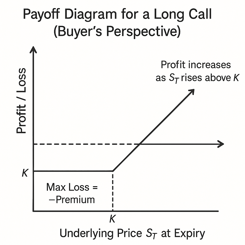
| Call | Buy the asset | $\max(S_T - K, 0)$ | Profitable if the final asset price ($S_T$) is above the strike price ($K$). |
| Put | Sell the asset | $\max(K - S_T, 0)$ | Profitable if the final asset price ($S_T$) is below the strike price ($K$). |
The premium is the upfront price paid by the buyer to the seller (writer) for this right.
3 Birth of Black-Scholes—Replication Meets Calculus
In 1973, Fischer Black and Myron Scholes (with significant contributions from Robert Merton, who extended the model) published a groundbreaking paper. Their key insight was that an option’s payoff could be replicated by continuously trading a specific portfolio consisting of the underlying asset and risk-free borrowing/lending.
The idea is:
- Create a portfolio containing a certain amount ($\Delta$, or delta) of the underlying asset and some risk-free borrowing/lending.
- Continuously adjust the amount of the underlying asset ($\Delta$) held as its price changes, such that the portfolio’s value changes exactly mimic the option’s value changes over a very short time interval. This eliminates risk locally.
- Since this dynamically adjusted portfolio is momentarily risk-free, it must earn the risk-free interest rate ($r$) to prevent arbitrage opportunities.
Translating this “dynamic replication” argument into the language of stochastic calculus yields the Black-Scholes Partial Differential Equation (PDE):
<!–MATH_DISPLAY_3–>
Here, $V$ is the option value, $t$ is time, $S$ is the underlying asset price, $\sigma$ is the volatility of the asset’s returns, and $r$ is the risk-free interest rate.
Solving this PDE with the specific boundary condition for a European call option (i.e., its value at expiry $T$ must be $V = \max(S_T - K, 0)$) gives the famous closed-form Black-Scholes pricing formulas. The market finally had a rigorous, theoretically sound benchmark for option prices.
4 Opening the Toolbox—The Formula Itself
For a European call option on a non-dividend-paying underlying asset:
<!–MATH_DISPLAY_4–>
where:
<!–MATH_DISPLAY_5–>
<!–MATH_DISPLAY_6–>
For a European put option:
<!–MATH_DISPLAY_7–>
Alternatively, one can use put-call parity, a model-independent relationship: $C - P = S - K e^{-rT}$.
Component Breakdown:
| Symbol | Meaning | Where to Obtain | Explanation |
|---|---|---|---|
| $C$, $P$ | Price of the Call / Put option | Output of the Formula | The fair value according to the model. |
| $S$ | Current spot price of the underlying asset | Trading screen, market data feed | The current market price of the asset (e.g., stock price). |
| $K$ | Strike price (or Exercise price) | Option contract specifications | The fixed price at which the asset can be bought (call) or sold (put). |
| $T$ | Time to expiry (in years) | Calendar days until expiry ÷ 365 (or 365.25 / 252) | The remaining life of the option. Convention varies (365 vs 365.25 vs trading days ~252). |
| $r$ | Continuously compounded risk-free interest rate (annualised) | Government bond yield (e.g., Treasury), repo rate | The return on a risk-free investment over the option’s life. Must match the tenor $T$. |
| $\sigma$ | Volatility of the underlying asset’s returns (annualised std dev) | Historical data (historical vol) or market prices (implied vol) | Measures the expected magnitude of price fluctuations. Crucial input. |
| $e^{-rT}$ | Discount factor | Calculated from $r$ and $T$ | Converts the future strike price $K$ to its present value. |
| $\Phi(x)$ | Standard Normal Cumulative Distribution Function (CDF) | Statistical tables, Excel (NORM.S.DIST(x, TRUE)), code libraries |
Gives the probability that a standard normal random variable (mean=0, std dev=1) will be less than or equal to $x$. $d_1$ and $d_2$ act as standardised values. |
| $\ln(S/K)$ | Natural logarithm of the ratio of Spot to Strike | Calculated from $S$ and $K$ | Measures how far the option is in-the-money or out-of-the-money on a relative basis. |
Important Note: Ensure consistent units. $T$ must be in years, and $r$ and $\sigma$ must be annualised rates (e.g., 5% = 0.05). The term $\sigma\sqrt{T}$ scales the annual volatility to the time horizon of the option.
5 Worked Example—A One-Month Index Call
Let’s price a hypothetical call option on an index.
Parameters:
- Today’s Date: 28 April 2025
- Underlying Index Spot Price $S$: 22,500
- Strike Price $K$: 23,000 (This is an out-of-the-money call)
- Expiry Date: 28 May 2025 (30 days remaining)
- Time to Expiry $T$: $30 / 365 \approx 0.0822$ years
- Risk-Free Rate $r$: 7% per annum (continuously compounded) $\implies 0.07$
- Volatility $\sigma$: 15% per annum $\implies 0.15$
Step 1: Calculate Intermediate Values
- Volatility scaled by time: <!–MATH_DISPLAY_8–> (Note: Slight difference from original due to rounding $\sqrt{0.0822}$)
- Log of spot/strike ratio: <!–MATH_DISPLAY_9–>
- Risk-adjusted drift term: <!–MATH_DISPLAY_10–>
- Calculate $d_1$: <!–MATH_DISPLAY_11–>
- Calculate $d_2$: <!–MATH_DISPLAY_12–>
Step 2: Find Normal Probabilities (CDF Values)
Using a standard normal CDF calculator or function (like NORM.S.DIST in Excel):
- $\Phi(d_1) = \Phi(-0.3558) \approx 0.3610$
- $\Phi(d_2) = \Phi(-0.3988) \approx 0.3450$
Step 3: Calculate the Call Price ©
- Present value of strike price: <!–MATH_DISPLAY_13–>
- Plug into the Black-Scholes formula: <!–MATH_DISPLAY_14–> <!–MATH_DISPLAY_15–> <!–MATH_DISPLAY_16–> <!–MATH_DISPLAY_17–>
(Result is very close to the original ₹232.5; minor differences are due to rounding during intermediate steps).
Interpretation:
- The model suggests a fair price of ₹233.0 for this call option.
- Breakeven Price at Expiry: Strike Price + Premium = $23000 + 233.0 = 23233$. The index needs to rise above this level by expiry for the buyer to make a net profit.
- Maximum Loss: The premium paid (₹233.0) if the index finishes at or below 23000.
- Maximum Gain: Theoretically unlimited, as the index price can rise indefinitely.
Sensitivity: A small change in the volatility input ($\sigma$) can significantly impact the calculated price. If $\sigma$ were higher (e.g., 25% instead of 15%), the option price would increase substantially because higher volatility increases the chance of a large upward move (beneficial for a call option). This highlights why volatility forecasting is crucial in options trading.
6 Meet the Greeks—Sensitivity Dashboard
The “Greeks” are measures of an option’s sensitivity to changes in the underlying parameters. They are essential for risk management and hedging.
| Greek | Symbol | Definition | Practical Insight | Formula (Call) | Example Value (Illustrative) |
|---|---|---|---|---|---|
| Delta | $\Delta$ | $\frac{\partial C}{\partial S}$ | Change in option price per ₹1 change in spot price. Hedge ratio (how many shares to hold to hedge the option). | $\Phi(d_1)$ | 0.36 (from $\Phi(d_1)$ above) |
| Gamma | $\Gamma$ | $\frac{\partial^2 C}{\partial S^2}$ | Change in Delta per ₹1 change in spot price. Measures convexity risk. Highest for at-the-money (ATM) options near expiry. | $\frac{\phi(d_1)}{S\sigma\sqrt{T}}$ | 0.00007 (approx) |
| Vega | $\nu$ | $\frac{\partial C}{\partial \sigma}$ | Change in option price per 1% change in volatility. Sensitivity to vol changes. | $S \phi(d_1) \sqrt{T}$ | ₹98 (approx) |
| Theta | $\Theta$ | $\frac{\partial C}{\partial t}$ | Change in option price per day passing (time decay). Negative for long options (value erodes over time). | $-\frac{S\phi(d_1)\sigma}{2\sqrt{T}} - rKe^{-rT}\Phi(d_2)$ | -₹2.6 per day (approx) |
| Rho | $\rho$ | $\frac{\partial C}{\partial r}$ | Change in option price per 1% change in risk-free rate. More significant for longer-dated options. | $K T e^{-rT} \Phi(d_2)$ | ₹7.5 (approx) |
(Note: $\phi(x)$ is the standard normal probability density function (PDF), distinct from the CDF $\Phi(x)$.) Example values are roughly calculated based on the worked example parameters and are for illustration only.
Traders monitor these five numbers constantly, much like pilots watch their instruments (altitude, airspeed, heading, etc.), to understand and manage the risks of their option positions.
7 Beyond the Ivory Tower—Where Black-Scholes Bends
The Black-Scholes model is built on several simplifying assumptions that don’t always hold true in real markets. Recognizing these limitations is crucial:
- Constant Volatility Assumption vs. Volatility Smiles/Skews: The model assumes volatility ($\sigma$) is constant. In reality, implied volatility (volatility backed out from market prices) varies depending on the strike price and expiry. Deep out-of-the-money puts often have higher implied vols (“skew” or “smile”), reflecting market demand for crash protection, which contradicts the model.
- Continuous Price Movement vs. Jumps & Gaps: The model assumes prices move smoothly (log-normal diffusion). Real asset prices can gap or jump suddenly due to news (e.g., earnings announcements, geopolitical events). Models incorporating jumps (like Merton’s jump-diffusion model) or stochastic volatility (where vol itself changes randomly, like the Heston model) can sometimes provide better fits.
- No Transaction Costs or Taxes vs. Real-World Frictions: The model assumes continuous, costless hedging is possible. In reality, trading incurs brokerage fees, bid-ask spreads, and taxes, making perfect replication impossible and costly.
- Constant Interest Rates vs. Term Structure: The model assumes a single, constant risk-free rate ($r$). In reality, interest rates vary with maturity (the yield curve). Using different rates for options with different expiries might be necessary.
- Continuous Trading vs. Market Halts: The model assumes trading occurs continuously. Real markets have opening/closing times, holidays, and occasional halts (circuit breakers, liquidity freezes), during which hedging isn’t possible.
- Rational Pricing vs. Behavioural Biases: The model assumes all investors are rational. Behavioural finance suggests investors can be influenced by emotions and biases, sometimes leading to mispricings (e.g., persistent demand for lottery-like out-of-the-money calls might inflate their implied volatility).
Practical Approach: Use Black-Scholes as a foundational benchmark, but be aware of its limitations. Market practitioners often use implied volatility derived from market prices within the Black-Scholes framework, implicitly incorporating some market realities (like the vol smile) into the pricing.
8 Global Footprint and Ongoing Evolution
Despite its limitations, the Black-Scholes framework remains deeply embedded in finance:
- Risk Management: Value-at-Risk (VaR) models and other risk systems often use Black-Scholes (or variants) to value options within portfolios and estimate sensitivities (Greeks).
- Market Data & FinTech: Option chain displays on trading platforms and financial apps universally show implied volatility, which is calculated by inverting the Black-Scholes formula using observed market prices.
- New Markets: When new derivative markets emerge (e.g., for carbon credits, cryptocurrencies), Black-Scholes often serves as the initial default pricing model due to its tractability and familiarity.
- Basis for Advanced Models: More complex models (stochastic volatility, jump-diffusion, local volatility) often build upon or relate back to the Black-Scholes PDE and its core concepts.
- Computational Finance: Research continues into faster and more accurate ways to solve the Black-Scholes PDE or its extensions, including using techniques from AI (like neural networks to approximate pricing functions) and exploring quantum computing for complex derivatives.
9 Closing Thoughts—An Equation as Storyteller
Black-Scholes is more than just algebra; it’s a powerful narrative about how uncertainty (volatility), time, and the time value of money interact to determine the value of financial opportunities (options). Understanding it provides valuable insights:
- Investors: Can interpret changes in implied volatility as market sentiment indicators (e.g., rising put volatility might signal increasing fear). They can use the model to assess whether options seem cheap or expensive relative to their own forecasts.
- Founders & Executives: Can use variants of the model to value employee stock options (ESOPs) for accounting purposes and to set strike prices that are fair and motivating.
- Students: Can gain deep intuition by coding the formula and running “what-if” scenarios, observing how price changes as inputs vary. This hands-on practice builds understanding faster than passive reading.
- Regulators: Can use the framework to understand derivative market dynamics, promote transparency, and assess systemic risks related to large option positions.
A Practical Exercise: Go to a financial website with live option quotes (e.g., for Nifty or a specific stock). Pick three call options with the same expiry: one in-the-money (ITM, $S > K$), one at-the-money (ATM, $S \approx K$), and one out-of-the-money (OTM, $S < K$). Find the required inputs ($S, K, T, r$) and the market’s implied volatility ($\sigma$). Plug these into the Black-Scholes formula. Compare your calculated price to the actual market price (mid-point of bid/ask). The differences (pricing errors) often reveal market dynamics not captured by the basic model, such as volatility skew or liquidity premiums.
India gave the world zero and the decimal system; mastering the concepts behind five Greek letters ($\Delta, \Gamma, \nu, \Theta, \rho$) is a manageable, yet rewarding, next step in financial literacy.